Cluster Analysis

This tutorial will demonstrate analysis with k-means and k-medians from the cluster module. We will use matplotlib for visualization of data and results.

import heat as ht
import matplotlib.pyplot as plt

Spherical Clouds of Datapoints

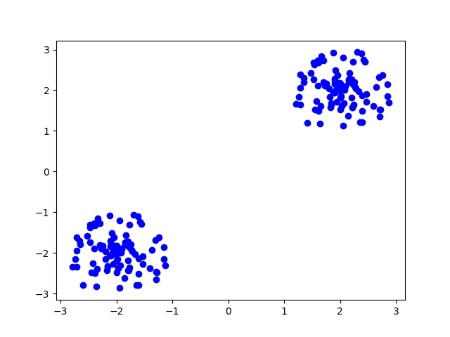
For a simple demonstration of the clustering process and the differences between the algorithms, we will create an artificial dataset, consisting of two circularly shaped clusters positioned at \((x_1=2, y_1=2)\) and \((x_2=-2, y_2=-2)\) in 2D space. For each cluster we will sample 100 arbitrary points from a circle with radius of \(R = 1.0\) by drawing random numbers for the spherical coordinates \(( r\in [0,R], \phi \in [0,2\pi])\), translating these to cartesian coordinates and shifting them by \(+2\) for cluster c1 and \(-2\) for cluster c2. The resulting concatenated dataset data has shape \((200, 2)\) and is distributed among the p processes along axis 0 (sample axis)

num_ele = 100
R = 1.0

# Create default spherical point cloud
# Sample radius between 0 and 1, and phi between 0 and 2pi
r = ht.random.rand(num_ele, split=0) * R
phi = ht.random.rand(num_ele, split=0) * 2 * ht.constants.PI

# Transform spherical coordinates to cartesian coordinates
x = r * ht.cos(phi)
y = r * ht.sin(phi)


# Stack the sampled points and shift them to locations (2,2) and (-2, -2)
cluster1 = ht.stack((x + 2, y + 2), axis=1)
cluster2 = ht.stack((x - 2, y - 2), axis=1)

data = ht.concatenate((cluster1, cluster2), axis=0)

Let’s plot the data for illustration. In order to do so with matplotlib, we need to unsplit the data (gather it from all processes) and transform it into a numpy array. Plotting can only be done on rank 0.

data_np = ht.resplit(data, axis=None).numpy()
if ht.MPI_WORLD.rank == 0:
    plt.plot(data_np[:,0], data_np[:,1], 'bo')
    plt.show()

This will render something like

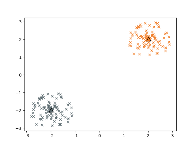
Now we perform the clustering analysis with kmeans. We chose ‘kmeans++’ as an intelligent way of sampling the initial centroids.

kmeans = ht.cluster.KMeans(n_clusters=2, init="kmeans++")
labels = kmeans.fit_predict(data).squeeze()
centroids = kmeans.cluster_centers_

# Select points assigned to clusters c1 and c2
c1 = data[ht.where(labels == 0), :]
c2 = data[ht.where(labels == 1), :]
# After slicing, the arrays are not distributed equally among the processes anymore; we need to balance
c1.balance_()
c2.balance_()

print(f"Number of points assigned to c1: {c1.shape[0]} \n"
      f"Number of points assigned to c2: {c2.shape[0]} \n"
      f"Centroids = {centroids}")

Number of points assigned to c1: 100
Number of points assigned to c2: 100
Centroids =  DNDarray([[ 2.0169,  2.0713],
                       [-1.9831, -1.9287]], dtype=ht.float32, device=cpu:0, split=None)

Let’s plot the assigned clusters and the respective centroids:

c1_np = c1.numpy()
c2_np = c2.numpy()

if ht.MPI_WORLD.rank == 0:
    plt.plot(c1_np[:,0], c1_np[:,1], 'x', color='#f0781e')
    plt.plot(c2_np[:,0], c2_np[:,1], 'x', color='#5a696e')
    plt.plot(centroids[0,0],centroids[0,1], '^', markersize=10, markeredgecolor='black', color='#f0781e' )
    plt.plot(centroids[1,0],centroids[1,1], '^', markersize=10, markeredgecolor='black',color='#5a696e')
    plt.show()

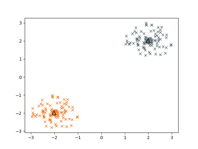
We can also cluster the data with kmedians. The respective advanced initial centroid sampling is called ‘kmedians++’.

kmedians = ht.cluster.KMedians(n_clusters=2, init="kmedians++")
labels = kmedians.fit_predict(data).squeeze()
centroids = kmedians.cluster_centers_

# Select points assigned to clusters c1 and c2
c1 = data[ht.where(labels == 0), :]
c2 = data[ht.where(labels == 1), :]
# After slicing, the arrays are not distributed equally among the processes anymore; we need to balance
c1.balance_()
c2.balance_()

print(f"Number of points assigned to c1: {c1.shape[0]} \n"
      f"Number of points assigned to c2: {c2.shape[0]} \n"
      f"Centroids = {centroids}")

Plotting the assigned clusters and the respective centroids:

c1_np = c1.numpy()
c2_np = c2.numpy()
if ht.MPI_WORLD.rank == 0:
    plt.plot(c1_np[:,0], c1_np[:,1], 'x', color='#f0781e')
    plt.plot(c2_np[:,0], c2_np[:,1], 'x', color='#5a696e')
    plt.plot(centroids[0,0],centroids[0,1], '^', markersize=10, markeredgecolor='black', color='#f0781e' )
    plt.plot(centroids[1,0],centroids[1,1], '^', markersize=10, markeredgecolor='black',color='#5a696e')
    plt.show()

The Iris Dataset

The _iris_ dataset is a well known example for clustering analysis. It contains 4 measured features for samples from three different types of iris flowers. A subset of 150 samples is included in formats h5, csv and netcdf in Heat, located under ‘heat/heat/datasets’, and can be loaded in a distributed manner with Heat’s parallel dataloader

iris = ht.load("heat/datasets/iris.csv", sep=";", split=0)

Fitting the dataset with kmeans:

k = 3
kmeans = ht.cluster.KMeans(n_clusters=k, init="kmeans++")
kmeans.fit(iris)

Let’s see what the results are. In theory, there are 50 samples of each of the 3 iris types

labels = kmeans.predict(iris).squeeze()

# Select points assigned to clusters c1 and c2
c1 = iris[ht.where(labels == 0), :]
c2 = iris[ht.where(labels == 1), :]
c3 = iris[ht.where(labels == 2), :]
# After slicing, the arrays are not distributed equally among the processes anymore; we need to balance
c1.balance_()
c2.balance_()
c3.balance_()

print(f"Number of points assigned to c1: {c1.shape[0]} \n"
      f"Number of points assigned to c2: {c2.shape[0]} \n"
      f"Number of points assigned to c3: {c3.shape[0]}")