Clustering and Principal Component Analysis (PCA)#

~1.4M Asteroids from the JPL Small Body Database#

[ ]:

from ipyparallel import Client
rc = Client(profile="default")
rc.ids

if len(rc.ids) == 0:
    print("No engines found")
else:
    print(f"{len(rc.ids)} engines found")

4 engines found

[ ]:

%%px
import heat as ht

Load the data from `hdf5` and preprocessing#

This has already been done in the respective notebook, so we skip the details and just proceed as follows:

[ ]:

%%px
from heat.preprocessing import StandardScaler
x = ht.load("/p/scratch/training2546/datasets/jplsbdb_asteroids.h5", "properties", device="gpu", split=0)
scaler = StandardScaler(copy=False)
scaler.fit_transform(x)

Out[2:7]: StandardScaler({})

Out[0:7]: StandardScaler({})

Out[1:7]: StandardScaler({})

Out[3:7]: StandardScaler({})

Clustering with K-Means#

Now, we will do the actual clustering:

[ ]:

%%px
from heat.cluster import KMeans
kmeans = KMeans(n_clusters=5, init="batchparallel")
kmeans.fit(x)
print(kmeans.labels_)

[stdout:2]

[stdout:1]

[stdout:3]

[stdout:0] DNDarray([[1],
          [0],
          [0],
          ...,
          [3],
          [1],
          [0]], dtype=ht.int64, device=gpu:0, split=0)

Visualization with PCA#

How do you know whether your results of clustering are meaningful? — You somehow need to visualize them. As most people (even mathematicians) might have problems visualizing point clouds in more than 4 dimensions (3D space + time), its a convenient option to use dimensionality reduction before vizualization.

Here, we will use PCA (“Principal Component Analysis”) for doing so. This technique relies on the mathematical concept of singular value decomposition (SVD); see the Linear Algebra notebook for more details.

[ ]:

%%px
from heat.decomposition import PCA
pca = PCA(svd_solver="full")
pca.fit(x)
print(pca.singular_values_)

[stdout:2]

[stdout:3]

[stdout:1]

[stdout:0] DNDarray([2.4105e+03, 1.4566e+03, 1.3290e+03, 1.3022e+03, 1.2496e+03, 1.1295e+03, 1.1131e+03, 1.0657e+03, 9.7940e+02,
          2.4479e+02, 7.0850e-01, 8.1861e-02], dtype=ht.float32, device=gpu:0, split=None)

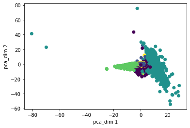
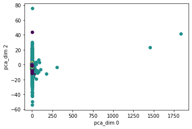
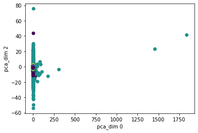
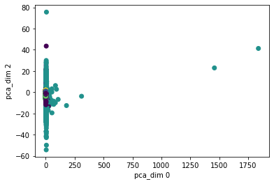
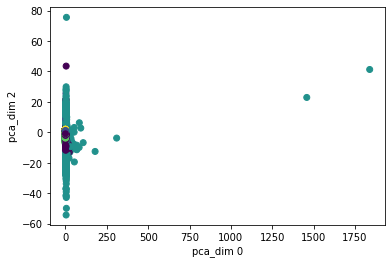
Once you have computed the PCA of your data, you can project onto the PCA-coordinates (pca.transform()) and plot the projected data points for various combinations of PCA-coordinates, here (1,2) and (0,2).

[ ]:

%%px
import matplotlib.pyplot as plt
%matplotlib inline

dim_list = [(1,2), (0,2)]
labels = kmeans.labels_.numpy()
for dims in dim_list:
    y = pca.transform(x)
    first_feature = y[:,dims[0]].numpy()
    second_feature = y[:,dims[1]].numpy()
    plt.figure()
    plt.scatter(first_feature, second_feature, c=labels)
    plt.xlabel(f'pca_dim {dims[0]}')
    plt.ylabel(f'pca_dim {dims[1]}')
    plt.show()